2011년 11월 30일 수요일

[자료] Fisher's Theory of Interest Rates and the Notion of 'Real': A Critique

자료: SSRN

By Eric Tymoigne, Lewis & Clark College
Levy Economics Institute Working Paper No. 483 , December 2006

※ Thanks to the author and the SSRN for providing the article on the Internet. This reader wants to study the content with some annotations and underlines, so anyone who is interested in it is kindly invited to visit the source link at the top.

※ Keywords: Real Interest Rate, Fisher
※ 검색어: Fisher, marginal rate of return over cost

Abstract:      

By providing five different criticisms of the notion of real rate, the paper argues that this concept, as Fisher defined it or as a definition, is not relevant to economic analysis. Following Keynes and other post-Keynesians, the article shows that the notion of real rate is microeconomically and macroeconomically unfounded. Adjusting interest rates for inflation does not protect the purchasing power of wealth, and it is impossible to do so at the macroeconomic level. In addition, an empirical interpretation of the break in the correlation between interest rates and inflation since 1953 is provided.


Fisher’s real rate of interest framework is essential for the inflation-targeting framework. It provides a rationale for the idea that monetary policy should be concerned mainly (if not only) with managing inflation expectations in order to keep real interest rates at a stable level that promotes saving and investment. Some post-Keynesians, like Smithin (2003) or Cottrell (1994), have also promoted the use of this concept, even if the former claimed that it only represents a definition and does not have anything to do with Fisher. Many authors have challenged the notion of real rate at the empirical level but only a few have done it at the theoretical level. Among those exceptions are authors like Keynes, Hahn, Harrod, Davidson, and Kregel.


The present article continues such critique and argues that the notion of real rate is not theoretically relevant for the study of micro- or macroeconomic problems—it does not protect against potential losses of purchasing power and the underlying arbitrage is impossible to do at the macroeconomic level. The paper also contributes to the large empirical literature on the subject by providing an interpretation of the break that occurred in the mid 1960s in the correlation between interest rates and inflation. In the end, we conclude that economic agents are far more concerned with nominal matters (i.e., financial power, or liquidity and solvency) than real problems (purchasing power). Not that the latter is ignored or unimportant, but it included into the broader considerations of the former.

The first four parts of the paper provide a theoretical criticism of Fisher’s theory, the fifth part of the paper provides an empirical study of the Fisher’s effect, and the paper concludes with an explanation of the relevance of nominal values.


1. ANTICIPATED INFLATION DOES NOT AFFECT NOMINAL INTEREST RATE

The first criticism of Fisher’s theory was provided by Keynes in the General Theory (1936). This criticism was restated and developed by Harrod (1971) and Davidson (1974, 1986). We know that, for Fisher, at the aggregate level:
i = r* + E(π)
Thus, given r* (the required real rate determined independently in the loanable funds market), any expected increase (decrease) in the rate of inflation will lead to an increase (decrease) in the nominal rate of interest via arbitrages between future and present aggregate incomes. Indeed, say that in time t = 0, the economy is at a full employment equilibrium with no inflation expected (i_0 = r*). Suddenly, in time t = 1, the central bank is expected to increase the money supply in time 2 so that, following the quantity theory of money, there is some inflation expected: E_1(π_2) = m_2 so that, in time 1, i_0 – E_1(π_2) < r*. Aggregate real income grows at a faster rate than the expected real amount of money that needs to be reimbursed (and so, too, the expected amount of real aggregate income to give up in the future if one borrows). The willingness to smooth consumption gives an incentive to borrow money now in order to buy some present income while giving up some future income. This puts an upward pressure on the money-rate on money:
If inflation is going on, he will see rising prices and rising profits, and will be stimulated to borrow capital unless interest rate rises; moreover, this willingness to borrow will itself raise interest rate. (Fisher 1907)
Theoretically, i should grow immediately to compensate for E_1(π_2) and no real effect should occur from the rise of money because the required and expected real rates are equal: i_1 – E_1(π_2) = r*, with i_1 > i_0.[주1]

[주1] Inflation will occur because of the increase in the money supply by the central bank.

Keynes was the first to have some difficulties with this explanation of the business cycle. His direct criticism rests on three points, with the third one being the consequences of the first two.
  • First, what should be compared are the money-rates, not the real rates, because the former are the only observable and the liquidity of position is essential—capital gain/loss should be included in the yield rate calculation.[주2]
  • Second, capital assets are usually not a good substitute for monetary assets as a store of value, whereas there is a high substitutability among monetary assets, and between monetary assets and liquid non-monetary assets. 
  • Third, for the two preceding reasons, Fisher’s explanation of what drives the interest rate on money is invalid. Changes in interest rates do not reflect changes in the opportunity cost induced by inflation in the present/future consumption arbitrage, they reflect changes in uncertainty that affect the stock equilibrium between liquid and illiquid assets. 
Stated alternatively:
The occurrence of a new-found belief firmly held, that a certain rate of inflation will occur, cannot affect the rate of interest. But the growth of uncertainty about what rate of inflation, if any, is in prospect, can send up the rate of interest. (Harrod 1971)
Let us look in detail at each criticism.
  • First, remember that there are three possible assets to choose from to hedge against inflation: money, bonds, and capital assets. At equilibrium, all three money-rates are equal and so no alternative is better than any other. Fisher’s theory assumes that r* is fixed for given time-preference and technology, and represents what people ultimately want—goods to consume. Of course, r* does not depend on the actual price of the asset because it is a required physical rate fixed by technology and tastes. However, the price of assets matters for the purchasing power—either directly by affecting the total return obtained after selling an asset or indirectly by affecting the creditworthiness of the asset owner. Thus, the arbitrage analysis should not start with real rate and go to nominal rate, but should start directly with nominal rates and compare cash outflows to cash inflows.
  • Second, “so long as it is open to the individual to employ his wealth in hoarding or lending money, the alternative of purchasing actual capital assets cannot be rendered sufficiently attractive (especially to the man who does not manage the capital assets and knows very little about them), except by organizing markets wherein these assets can be easily realised for money” (Keynes 1936). Usually, capital assets are illiquid so that they cannot be resold at all or only by recording large capital losses. Thus, illiquid capital assets are “not […] a hedge against inflation and hence will be shunned by savers” (Davidson 1986, italics added). This, of course, goes against the more recent Monetarist development of Fisher’s theory that assumes that the relevant transmission mechanisms of a monetary shock goes beyond the portfolio adjustments in terms of financial assets to include also “such assets as durable and semi-durable consumer goods, structures, and other real property” like “houses, automobiles, […] furniture, household appliances, clothes, and so on” (Friedman 1974).
  • The third and essential criticism of Fisher by Keynes is delivered in the following way:
There is no escape from the dilemma that, if it is not foreseen, there will be no effect on current affairs; whilst, if it is foreseen, the prices of existing goods will be forthwith so adjusted that the advantages of holding money and of holding goods are again equalized, and it will be too late for holders of money to gain or suffer a change in the rate of interest which will offset the prospective change during a period of the loan in the value of the money lent. For the dilemma is not successfully escaped by Professor Pigou’s expedient of supposing that the prospective change in the value of money is foreseen by one set of people but not foreseen by another. (Keynes 1936)
Thus, in any case, in the context of Fisher’s theory, the money holders (the lenders) will never be able to adjust the interest rate, i.e., the interest rate on bonds, before inflation occurs. After inflation occurred, money holders will not have any incentive to do any arbitrage because all money-rates will be equal again. In order to understand why, it is first necessary to understand how the rate of interest could go up because of perfectly expected inflation. This would not result from an arbitrage between money and bonds because both are monetary assets and so both are affected exactly in the same way by inflation:
Bonds and cash are two forms of asset denominated in money. Neither has a hedge against inflation. […] The rate of interest represents the rate at which bonds can be exchanged for cash. Since neither contains a hedge against inflation, the new-found expectation that inflation will occur cannot change their relative values or therefore, the rate of interest. […] The idea that new-found expectation can alter the relative value of two money-denominated assets, is logically impossible, and must not be accepted into the corpus of economic theory. (Harrod 1971)
The only reason why the interest rate would go up is because individuals want to switch their portfolio from monetary assets to liquid non-monetary assets. The problem is, then, to know if they actually can do this arbitrage based on perfectly expected inflation. Keynes’s answer is no. Indeed, on one side, if inflation was not foreseen (if neither borrowers nor lenders saw that a monetary shock occurred and so thought that i_0 = r*), then lenders did not have any incentive to raise the rate of interest and borrowers did not have any incentive to borrow. Once inflation occurred, those who are long in monetary assets record an unexpected loss in real terms (i_0 – π_2 < r*), whereas those who are long in capital assets record an unexpected gain in nominal terms (i_0 < r* + π_2); it is too late to make up for inflation—money holders record a loss that cannot be avoided by increasing i. At the same time, there is no more incentive for monetary-asset holders to do any more arbitrages because i_0 = r* again (assuming that no more inflation is expected).

(...) 

3. THE TRANSFER OF REAL INCOME OVER TIME

Fisher assumes that the arbitrage that goes on at the microlevel between present and future income can be applied at the macroeconomic level with aggregate real income. This has, again, been criticized by Keynes (1936):
Aggregate demand can be derived only from present consumption or from present provision for future consumption. The consumption for which we can profitably provide in advance cannot be pushed indefinitely into the future. We cannot, as a community, provide for future consumption by financial expedients but only by current physical output. In so far as our social and business organisation separates financial provision for the future from physical provision for the future so that efforts to secure the former do not necessarily carry the latter with them, financial prudence will be liable to diminish
aggregate demand and thus impair well-being, as there are many examples to testify. (Keynes 1936, italics added)
Thus, not only is Fisher’s condition of indifference wrong at the microlevel, it is also wrong at the aggregate level.
  • In the former case, it does not automatically protect individuals against purchasing power loss, and 
  • in the second case, arbitrage is impossible because there are no spot and forward markets for a “commodity” called “aggregate income.” 
Therefore, saving can only come in monetary terms, not in real terms. However, saving in financial terms today does not lead automatically to the production or the provision for the production of future goods and services. The only way to save for the future in real terms is to invest today.

Actually, in his own terms, Fisher seems aware of this. He recognizes that a person can change his/her real income streams in two ways (Fisher 1930)—via their impatience (borrowing and lending) and via investment. However, at the aggregate level, the first solution is not possible:
Borrowing and lending, the narrower method of modifying income streams, cannot be applied to society as a whole, since there is no one outside to trade with; and yet society does have opportunities radically to change the character of its income stream by changing the employment of its capital. (Fisher 1930)

Stated alternatively, the arbitrage process that leads to the condition of indifference cannot be applied at the aggregate level. Or, again, the loanable funds supply and demand functions do not exist at the aggregate level. He should have concluded that the market interest rate cannot be determined in this way, but he did do so and instead continued his analysis by assuming that all the results obtained from microeconomic reasoning apply at the macroeconomic level.


4. THE THEORY OF RATE OF INTEREST

Keynes (1937, 1936), Kregel (1988, 1999), and Kahn (1984) already made a criticism based on the same lines. Fisher assumes that r* is given by technology and tastes. r* is a physical rate of return. However, in his analysis, Fisher recognizes that r* is actually calculated in money terms and that price expectations matter for the decision—the rate of return over cost is the monetary expression of r* and is the essential variable for investment (Fisher 1930). Later, Keynes explicitly stated that the marginal efficiency of capital and the rate of return are identical concepts. One could then wonder if it is justified
to criticize Fisher’s analysis for not taking into account the importance of money and monetary expectations.


In fact, in Fisher’s theory, money is a veil and Keynes should not have confounded marginal efficiency of capital and marginal rate of return over cost as depicted by Fisher. Indeed, in Fisher, the real return is guaranteed because it depends on the technical capacity of the productive assets. Stated alternatively, the rate of return over cost is concerned with the “profit” obtained from the produced output expressed in monetary terms, whereas the marginal efficiency of capital is concerned with the profit obtained from the sale of the production. This should be clear if one reads the following quote:


In the real world our options are such that if present income is sacrificed for the sake of future income, the amount of future income secured thereby is greater than the present income sacrificed. […] Man can obtain from the forest or the farm more by waiting than by premature cutting trees or by exhausting the soil. […] Nature offers man may{many} opportunities for future abundance at trifling present cost. So also human technique and invention tend to produce big returns over cost. (Fisher 1930, italics added)


Thus, the rate of return is just a monetary expression of the “primitive cost and return typified by labor and satisfaction” (Fisher 1930). On the other side, Keynes was very careful to state that the marginal efficiency of capital does not rest directly on technical concepts (Kregel 1988): “If capital becomes less scarce, the excess yield will diminish, without its having become less productive—at least in the physical sense” (Keynes 1936).


5. THE FISHER INDIFFERENCE CONDITION AS A DEFINITION

Some post-Keynesian authors, like Smithin (2003) or Cottrell (1994), even if they reject the notion of real rate of return, agree that the real rate of interest is a useful concept in terms of definition:
Interest rates are determined in the financial sector proximately by the decision of the ultimate provider of credit, in other words the central bank. This institution also sets the pace for real interest rates, and not just for nominal rates. The real interest rate (on Fisher’s definition) is just the nominal rate minus expected inflation. Hence the central bank can set the real rate, if it wishes, simply by adjusting the setting of the nominal rate to offset changes in expectation of inflation (Smithin 2003).
This position is, however, quite problematic for several reasons. First, it puts a real concept into the monetary framework. It is the relationship between nominal cash inflows and nominal cash outflows that matters, rather than the notion or “real” income. “Real” assumes that cash outflows are only linked to consumption and that the cash outflows of different economic agents are equally affected by inflation. It does not take into account the fact that the structure of spending, as well as financial commitments, are crucial for the effect of prices on cash-outflows. As Pigeon notes, for example, unionized workers in Canada have wage demands that “are anchored on expected inflation and interest rates” (Pigeon 2004). In itself, the real wage is an inefficient way to protect the purchasing power of wage; the whole range of cash outflows should be accounted for so as to protect the financial power of wage. It is the same with financial income earners whose consumption outflow is far less important in proportion than cash outflows due to financial commitments like interest, margin calls, or off-balance sheet commitments.


Second, the idea that Fisher’s real rate of interest is “just” a definition is not what Fisher had in mind. Fisher’s indifference condition reflects a hypothesis about the behavior of individuals and their method of selecting assets. It also reflects a particular conception of income (Kregel 1999). However, as shown above, this condition is problematic for several reasons. In addition, if one assumes that the real rate of interest is just a definition, one must assume that there is a clear correlation between inflation and nominal interest rates. However, as shown above, Fisher was the first to recognize that this is not the case. In fact, many studies, including Fisher, have shown that the “Fisher effect” does not hold.[주7] The following confirms the conclusion of Fisher. The analysis is divided in two parts. In the first part, the correlation between variables are checked and some conclusions are drawn. In the second part, a Granger causality test is performed to substantiate the previous conclusions.


5.1. Analysis of Correlations

(...) 


2011년 11월 29일 화요일

[Schumpeter's comment on] Fisher's marginal rate of return over cost

자료: 구글도서

※ 메모:

(... de)cision at the hands of Keynes. As everyvody knows, it represents current total national consumption(total expenditure on 'consumption' in terms of wage units) as a function of current national income (in wage units) and expresses the arbitrary postulate that any increase in the latter is always attended by an increase in the former but by a smaller one.[주13] The investment function is less easy to convey in a few words because of its connection with the very important dynamical considerations of Keynes's chapter 11 and 12, which do not enter into its explicit statement. It relates the rae of aggregate investment to the marginal efficiency of (physical) 'capital in general which that rate of investment will establish' (op. cit. p. 136), the marginal efficiency of capital being defined as the relation between the expected yield of one more unit (properly chosen) of any capital good and the cost of producing this unit.[주14]. This, as Keynes pointed out, is the same as Fisher's 'marginal rate of return over cost.'[주15] But there is this difference between the two : whereas with Fisher this marginal rate of return over costㅡwhich implies a discounting process of the series of expected yieldsㅡconstitutes the basic fact about the interest phenomenon, Keynes broke away at this point from what I have termed the Barbon tradition and, in intent at least, established a monetary theory of interest, according to which interest is not derived from, or expressive of, anything that has, in whatever form, to do with the net return from capital goods.[주16]

(...)

[주15] ^Theory of Interest^(1930), p. 168. I can, however, testify to the fact that Keynes, whose knowledge of economic literature and particularly of contemporaneous and non-English literature was not of the first order, arrived at his concept quite independently and that he inserted the acknowledgment in question upon his attention's having been drawn to Fisher's formulation. When he received the information, Keynes possibly ackwowledged too much. Such, at least, is Professor Lerner's opinion. On the other hand, it may be argued that both concepts are indeed improvements upon the concept of marginal productivity of capital as developed by Marshall and especially Wicksellㅡand this again points back to Bohm-Bawerkㅡbut not more than that. The 'prospectiveness' of marginal productivity of capital and its relation to its replacement costs, few if any authors who used it would have denied.

[자료] Keynsian Teachings: Past and Present


※ Key words: marginal rate of return over cost, in Irving Fisher

※ 발췌: 

(...) Any new investment achieved by an economic operator will determine the salary increase for all employees engaged in business activities (the wage is tied to the marginal cost of labor of the last worker employed). This should result in an increase in annuity rates of return due to increase of aggregate demand. This phenomenon may represent in a particular case a Keynesian condition for achieving investment if it is based on credit because rising demand for loans (at the macro level) or indebtedness (of an economic agent) will strengthen interest rate level. [4] So while the marginal profit of each plant decreases (by market share increasingly lower production level of the individual) investment position remains firm at a constant slope.

The explanation for this phenomenon can be found in Irving Fisher's theory of "Nature of Capital and Income" (1906), "Rate of Interest" (1907) and especially in the important work of his "Theory of Interest" (1930) which show that the investment function is especially a problem of inter-temporal decision. According to his opinion, investment function is as follows:
V2=f(L,I1) where:
V2 representing the investment incomes
L labour force is a constant
I1 achieved investment
As an investment generates money after having been fully achieved, we must take into account two successive periods t1, the establishing term of investment and t2 the period of establishing investments. How labor costs is a constant, it means that incomes depend on the costs of the investment, so the function becomes: V2=f(I1).

If interest rate is d` we can say that it will influence the investment function at the level (1+d`)I1, which possibly implies the amount of interests paid by the company when achieving investments by credits. Investment profit is represented by:
π=f(I1)- (1+d`)I1
Its maximization is reached when:
f `=(1+d`)
What for Fisher ”f `-1” represents the marginal profit that exceeds the cost ("marginal rate of return over cost") in the Keynesian theory, the name of the marginal investment is marginal efficiency of investment. It is obvious (as in the Keynesian theory) the existence of a negative relationship between interest rate and the volume of investment. This theory generates many problems mainly because it does not address situations in which the contractor does not depend on loans to finance investment or the company is to maximize short term profit, lacking a strategic vision. According to Fisher, the capital is intended for all production processes, there is no capital stock or withdrawal under form of profit distribution to shareholders.

This issue was under discussion by Friedrich August von Hayek in his "Pure Theory of Capital" (1941). For him, (...)

2011년 11월 27일 일요일

[자료] 등비수열의 합

자료: http://en.wikipedia.org/wiki/Geometric_series


(...) The sum of a geometric series is finite as long as the terms approach zero; as the numbers near zero, they become insignificantly small, allowing a sum to be calculated despite the series being infinite. The sum can be computed using the self-similarity of the series.

[edit]Example


self-similar illustration of the sum s. Removing the largest circle results in a similar figure of 2/3 the original size.
Consider the sum of the following geometric series:
s \;=\; 1 \,+\, \frac{2}{3} \,+\, \frac{4}{9} \,+\, \frac{8}{27} \,+\, \cdots
This series has common ratio 2/3. If we multiply through by this common ratio, then the initial 1 becomes a 2/3, the 2/3 becomes a 4/9, and so on:
\frac{2}{3}s \;=\; \frac{2}{3} \,+\, \frac{4}{9} \,+\, \frac{8}{27} \,+\, \frac{16}{81} \,+\, \cdots
This new series is the same as the original, except that the first term is missing. Subtracting the new series (2/3)s from the original series cancels every term in the original but the first:
s \,-\, \tfrac23s \;=\; 1,\;\;\;\;\;\;\;\;\mbox{so }s=3.
A similar technique can be used to evaluate any self-similar expression.

[edit]Formula

a + ar + a r^2 + a r^3 + \cdots + a r^{n-1} = \sum_{k=0}^{n-1} ar^k= a \, \frac{1-r^{n}}{1-r},
where a is the first term of the series, and r is the common ratio. We can derive this formula as follows:


\begin{align}
&\text{Let }s = a + ar + ar^2 + ar^3 + \cdots + ar^{n-1}. \\[4pt]
&\text{Then }rs = ar + ar^2 + ar^3 + ar^4 + \cdots + ar^{n}  \\[4pt]
&\text{Then }s - rs = s(1-r) = a-ar^{n},\text{ so }s = a \frac{1-r^{n}}{1-r}.
\end{align}
The formula follows by multiplying through by a.
As n goes to infinity, the absolute value of r must be less than one for the series to converge. The sum then becomes
s \;=\; \sum_{k=0}^\infty ar^k = \frac{a}{1-r}=a+ar+ar^2+ar^3+ar^4+\cdots.
When a = 1, this simplifies to:
1 \,+\, r \,+\, r^2 \,+\, r^3 \,+\, \cdots \;=\; \frac{1}{1-r},
the left-hand side being a geometric series with common ratio r. We can derive this formula:

\begin{align}
&\text{Let }s = 1 + r + r^2 + r^3 + \cdots. \\[4pt]
&\text{Then }rs = r + r^2 + r^3 + \cdots. \\[4pt]
&\text{Then }s - rs = 1,\text{ so }s(1 - r) = 1,\text{ and thus }s = \frac{1}{1-r}.
\end{align}
The general formula follows if we multiply through by a.


This formula is only valid for convergent series (i.e., when the magnitude of r is less than one). For example, the sum is undefined when r = 10, even though the formula gives s = −1/9.
This reasoning is also valid, with the same restrictions, for the complex case.

(...)


Economics

In economics, geometric series are used to represent the present value of an annuity (a sum of money to be paid in regular intervals).
For example, suppose that you expect to receive a payment of $100 once per year (at the end of the year) in perpetuity. Receiving $100 a year from now is worth less to you than an immediate $100, because you cannot invest the money until you receive it. In particular, the present value of a $100 one year in the future is $100 / (1 + I), where I is the yearly interest rate.
Similarly, a payment of $100 two years in the future has a present value of $100 / (1 + I)2 (squared because it would have received the yearly interest twice). Therefore, the present value of receiving $100 per year in perpetuity
\sum_{n=1}^\infty \frac{\$100}{(1+I)^n}
can be expressed as an infinite series:
\frac{\$ 100}{1+I} \,+\, \frac{\$ 100}{(1+I)^2} \,+\, \frac{\$ 100}{(1+I)^3} \,+\, \frac{\$ 100}{(1+I)^4} \,+\, \cdots.
This is a geometric series with common ratio 1 / (1 + I). The sum is
\frac{a}{1-r} \;=\; \frac{\$ 100/(1+I)}{1 - 1/(1+I)} \;=\; \frac{\$ 100}{I}.
For example, if the yearly interest rate is 10% (I = 0.10), then the entire annuity has a present value of $1000.
This sort of calculation is used to compute the APR of a loan (such as a mortgage loan). It can also be used to estimate the present value of expected stock dividends, or the terminal value of a security.

(...)

2011년 11월 25일 금요일

[간략 복습] 주택저당담보증권(MBS), 자산담보부증권(ABS)

자료: 주택저당담보증권 (오마이뉴스, 2006.08.05)


(...) '저당의 유동화'란 저당권을 하나의 상품처럼 팔 수 있게 하는 것을 말합니다. 

예를 들어 차입자가 자신의 주택에 저당권을 설정하고 은행(대출자)으로부터 자금을 차입했습니다. 은행은 많은 자금을 확보해서 주택금융을 시작했지만, 주택금융이란 것이 고액을 장기로 융자하는 것이다 보니 어느 정도 시간이 지나면 은행의 자금(융자 자금)이 부족해지는 상황이 올 수 있습니다. 

이 때 은행의 자금부족 문제를 해결하기 위한 수단으로 나온 것이 바로 '저당의 유동화'입니다. 즉, 은행(대출자)이 가지고 있는 저당권을 2차 대출기관에게 팔아서 부족한 현금을 보충하자는 것입니다.

이제 본론으로 들어가서 주택저당담보증권(MBS)에 대해서 말씀드리겠습니다. 

[의의]
주택저당담보증권은 말 그대로 주택저당을 담보로 해서 발행한 증권입니다.

[발행 구조]
은행이 주택자금을 대출하고 취득한 '주택저당채권'을 유동화전문회사에게 양도합니다. 유동화전문회사란 은행의 주택저당채권을 전문으로 사주는 회사를 말하는데 우리나라에는 '한국주택금융공사'가 있습니다.

유동화전문회사는 자신이 사들인 주택저당채권을 기초로 증권을 발행하여 투자자들에게 매각하게 되는데, 이 증권을 주택저당담보증권이라고 합니다.

[발행의 효과]
은행은 유동화전문회사에 자신들이 가지고 있는 저당채권을 팔아서 주택금융에 필요한 자금을 조달합니다. 이렇게 되면 은행은 적은 자금을 가지고도 많은 차입자에게 대출을 해줄 수 있게 됩니다. 차입자 입장에서는 그만큼 주택자금 대출이 쉬워진다는 것을 의미합니다. 따라서 주택담보증권의 발행으로 무주택서민의 주택구입이 그 만큼 쉬워지고 확대될 수 있습니다.

투자자 입장에서는 한국주택금융공사에서 발행한 MBS에 투자해 보시는 것도 좋을 것 같습니다. 다른 부동산투자에 비해 투자위험이 상대적으로 적습니다.

참고로 한국주택금융공사는 다음과 같은 업무를 수행하고 있습니다.

① 모기지론(보금자리론) 공급: 만기 10년 이상의 장기저리 모기지론(보금자리론)을 공급하고 있습니다.

② 주택저당담보증권(MBS) 발행: 은행으로부터 저당채권을 사들여서 주택저당담보증권을 발행합니다.

③ 주택신용보증 업무: 서민 주거안정을 위해 전세자금 대출보증, 중도금 대출보증 업무를 하고 있습니다.

④ 대학생 학자금대출업무
(...) 

자료: HF공사, MBS 8062억원 발행 (아시아경제, 2011.11.24) 

한국주택금융공사(HF공사)는 "경남은행 등 14개 금융기관에서 취급한 보금자리론을 기초자산으로 총 8062억 원 규모의 주택저당증권(MBS)을 발행했다"고 24일 밝혔다.

이번에 발행된 MBS는 각각 1년에서 20년 만기의 선순위 8개 종목과 HF공사가 보유하는 21년 만기 후순위 1개 종목으로 구성됐으며, 기초자산인 주택담보대출의 조기상환에 대비해 만기 5년 이상의 종목에는 콜옵션을 부여했다.

이번에 발행된 MBS의 만기별 발행금리는 1년물 3.65%, 3년물 3.89%, 5년물 4.00%, 10년물 4.08%, 20년물 4.22%로 결정됐다.

한편, HF공사는 현재까지 85회에 걸쳐 총 37조 2681억원의 MBS를 발행했다


ABS (Asset Backed Securities): 말 그대로 자산을 근거로 하는 증권 입니다.무슨 자산을 근거로 하는냐. 무슨 자산이든 돈 될만한 것을 근거(정확히 말하면 담보)로 하는 증권입니다. 제가 님에게 돈을 빌리고 싶습니다. 님은 저에게 담보를 요구하겠죠. 그리고 저는 담보로 될만한 것을 님에게 제공하고 님에게 돈을 빌려야 님이 그나마 안전장치를 마련하게 되는 것이니 쉽게 돈을 빌려 주겠지요. 예를 들어 저에게 100만원 정도 가치를 지닌 금반지가 있습니다. 제가 돈이 50만원이 필요하면.. 님에게 금반지를 담보로 제공하고 50만원을 빌리겠지요. 그리고 50만원과 약속한 이자를 갚으면.. 님은 금반지에 대한 담보를 풀어줄 것입니다. 만일 돈을 갚지 않으면.. 금반지를 님은 경매 처분하여 자금을 회수하시면 됩니다.

그럼 기업이 ABS를 발행하는 것에 대해 간단 설명. 님이 옷을 만드는 회사를 한다고 가정하지요. 현재 님은 옷을 외상으로 5억원을 도매상에 팔았습니다. 그런데 현재 돈이 3억원이 필요합니다. 이런 경우.. 님은 돈을 가진 사람에게 갑니다. 그리고 외상매출채권을 담보로 잡히고 3억원을 빌려달라고 이야기합니다. 그리고 돈을 가진 사람은 님의 외상매출채권을 담보로 돈을 빌려줍니다. 이 때 계약서를 쓰겠지요. 이 계약서가 ABS라고 보시면 됩니다.

정확하게는 여러 사람에게 외상매출채권을 담보로 돈을 빌리게 되죠. 홍길동에게 3천만원, 감동이에게 1억원, 영삼이에게 5천만원... ... 등등등... 빌려서 3억원의 돈을 마련하고.. 각각에게 증서를 발행해 줍니다. 이것이 ABS 자산담보부증권 입니다. 

예전에 기업들은 돈이 필요하면.. 은행에 담보를 제공하고 돈을 빌려쓰곤 했는데.. 외환위기 이후... 은행이 기업에 대한 대출을 강화(BIS 비율을 맞춘다는 명목아래..)하면서... 기업들이 새롭게 자금조달을 위한 창구가 필요하게 되었습니다. 이런 이유에서 점차 발달하게 된 것이 ABS 시장입니다. 카드사의 외상매출채권을 담보로 발행을 하기도 하고, 강남의 빌딩을 가진 회사가 빌딩을 담보로 발행하기도 하고, 음반판권을 지닌 회사가 음반 판권을 담보로 발행하기도 합니다. 아무래도 담보를 제공하기 때문에 이자를 적게 줄 수 있고, 돈의 가치는 지니지만.. 당장 현금화 할 수 없는 자산을 이용해서 유동성을 강화시킨다는 측면이 긍정적이라고 할 수 있죠.

* MBS(주택저당담보증권)은 담보로 잡는 자산이 주택(모기지)이라는 것만 다릅니다. 크게 보면 MBS가 ABS에 포함이 된다고 보시면 됩니다. 님이 1억원 짜리 집을 사고 싶습니다. 돈이 5천만원 밖에 없습니다. 이런 경우 통상적으로 집을 구입하는 방법은 일단 님이 다른 사람에게 5천만원을 빌려 옵니다. 그리고 1억원짜리 집을 사죠. 그리고 은행에 가서 집을 담보로 5천만원을 빌립니다. 그리고 5천만원을 빌려온 사람에게 갚죠. 그리고 은행에 5천만원을 원금과 이자를 계속 갚아나갑니다. 이것이 이론적인 MBS죠. 집을 담보로 은행에서 돈을 빌리고 은행에 집을 담보로 한다는 것을 쓴 계약서가 이론적으로는 MBS라고 볼 수 있습니다.

그러나 현재 이야기 되고 있는 MBS는 이보다 한단계를 더 거치게 됩니다. 은행의 경우 장기로 돈을 빌려주는 것이 쉽지 않습니다. 장기로 돈을 넣어두는 사람(예금자)이 많지 않기 때문이기도 하지만.. 장기 금리기 어떻게 변할지 몰라서 장기로 돈을 빌려주고 싶어하지 않죠. 그래서 은행은 돈을 빌려 주고 잡은 담보를 다시 이용하여.. 새로운 증서를 발행하게 됩니다. 그리고 다른 사람에게 돈을 빌려 오는 것이죠. 현재 이것을 MBS라고 이야기합니다.

님은 집을 담보로 은행에서 돈을 빌리고. 은행은 그 집을 다른이에게 담보로 제공하여 돈을 회수하여.. 장기유동성제약에서 벗어나게 되죠. (네이버 "bigsea21" 님)

[자료] The Distribution of Wealth


지은이: 
James B. Davies (Department of Economics, University of Western Ontario, London N6A 5C2, Canada), & 
Anthony F. Shorrocks (Department of Economics, University of Essex, Colchester CO4 3SQ, UK)


※ 메모:  

This chapter surveys what is known about the distribution of personal wealth and its evolution over time. We review the descriptive evidence as well as theoretical and applied research that attempts to explain the main features of wealth-holdings and wealth inequality observed in the real world.

There are many reasons for interest in personal wealth, and many ways in which the concept of wealth may be defined. If we were concerned with the overall distribution of economic well-being or resources, it would be appropriate to examine the distribution of “total wealth”, that is, human plus non-human capital. But that is not our objective here. Instead, we exclude the human capital component and focus on material assets in the form of real property and financial claims. The term “wealth” will therefore usually refer to “net worth” — the value of non-human assets minus debts. Our aim is to examine the reasons for holding wealth, to document the observed differences in holdings across individuals and families, and to examine the causes of these observed differences.

(...)

The concept of net worth may appear to be straightforward, but should we deal with intangible assets which cannot be readily bought and sold? This category covers pension rights, life insurance, and entitlement to future government transfers (including “social security wealth”). Any attempt to include the rights to uncertain future benefits has to confront a variety of difficult valuation problems. For example, it is not obvious what discount rates should be used for these assets. Should they be risk-adjusted? Should a special adjustment be made for people who are borrowing constrained? Satisfactory answers to these questions require a considerable amount of painstaking work. It is therefore not surprising to discover that most applied work on wealth-holdings and wealth distribution confines itself to marketable wealth. When reviewing the empirical evidence, we use the term “augmented wealth” to refer to the broader concept which includes entitlements to future pension streams.

There are certain important “stylized facts” about the distribution of wealth which it is useful to highlight at the outset. These are:

1.  Wealth is distributed less equally than labour income, total money income or consumption expenditure. While Gini coefficients in developed countries typically range between about 0.3 and 0.4 for income, they vary from about 0.5 to 0.9 for wealth. Other indicators reveal a similar picture. The estimated share of wealth held by the top 1 percent of individuals or families varies from about 15-35 percent, for example, whereas their income share is usually less than 10 percent.

2.  Financial assets are less equally distributed than non-financial assets, at least when owner-occupied housing is the major component of non-financial assets. However, in countries where land value is especially important, the reverse may be true.

3.  The distribution of inherited wealth is much more unequal than that of wealth in general.

4.  In all age groups there is typically a group of individuals and families with very low net worth, and in a number of countries, including the United States, the majority havesurprisingly low financial assets at all ages.

5. Wealth inequality has, on the whole, trended downwards in the 20th century, although there have been interruptions and reversals, for example in the United States where wealth inequality has increased since the mid 1970s.

Possible explanations for these, and other, stylized facts will be investigated in this chapter. (...) 

[자료] U.S. Net Worth and the Assets of Households: 2002

자료: http://www.census.gov/prod/2008pubs/p70-115.pdf ( Census Bureau, Issued April 2008 )

※ 메모: Key Definitions and Explanation

[자료] Wealth, Income, and Power

자료: http://www2.ucsc.edu/whorulesamerica/power/wealth.html
by G. William Domhoff

This document presents details on the wealth and income distributions in the United States, and explains how we use these two distributions as power indicators. (...)

First, though, some definitions. Generally speaking, wealthis the value of everything a person or family owns, minus any debts. However, for purposes of studying the wealth distribution, economists define wealth in terms ofmarketable assets, such as real estate, stocks, and bonds, leaving aside consumer durables like cars and household items because they are not as readily converted into cash and are more valuable to their owners for use purposes than they are for resale (see Wolff, 2004, p. 4, for a full discussion of these issues). Once the value of all marketable assets is determined, then all debts, such as home mortgages and credit card debts, are subtracted, which yields a person's net worth. In addition, economists use the concept of financial wealth -- also referred to in this document as "non-home wealth" -- which is defined as net worth minus net equity in owner-occupied housing. As Wolff (2004, p. 5) explains, "Financial wealth is a more 'liquid' concept than marketable wealth, since one's home is difficult to convert into cash in the short term. It thus reflects the resources that may be immediately available for consumption or various forms of investments."

We also need to distinguish wealth from income. Income is what people earn from work, but also from dividends, interest, and any rents or royalties that are paid to them on properties they own. In theory, those who own a great deal of wealth may or may not have high incomes, depending on the returns they receive from their wealth, but in reality those at the very top of the wealth distribution usually have the most income. (But it's important to note that for the rich, most of that income does not come from "working": in 2008, only 19% of the income reported by the 13,480 individuals or families making over $10 million came from wages and salaries. See Norris, 2010, for more details.)

This document focuses on the "Top 1%" as a whole because that's been the traditional cut-off point for "the top" in academic studies, and because it's easy for us to keep in mind that we are talking about one in a hundred. But it is also important to realize that the lower half of that top 1% has far less than those in the top half; in fact, both wealth and income are super-concentrated in the top 0.1%, which is just one in a thousand. (To get an idea of the differences, take a look at an insider account by a long-time investment manager who works for the well-to-do and very rich. It nicely explains what the different levels have -- and how they got it. Also, David Cay Johnston (2011) has written a column about the differences among the top 1%, based on 2009 IRS information.)

(...)

So far there are only tentative projections -- based on the price of housing and stock in July 2009 -- on the effects of the Great Recession on the wealth distribution. They suggest that average Americans have been hit much harder than wealthy Americans. Edward Wolff, the economist we draw upon the most in this document, concludes that there has been an "astounding" 36.1% drop in the wealth (marketable assets) of the median household since the peak of the housing bubble in 2007. By contrast, the wealth of the top 1% of households dropped by far less: just 11.1%. So as of April 2010, it looks like the wealth distribution is even more unequal than it was in 2007. (See Wolff, 2010 for more details.)

There's also some general information available on median income and percentage of people below the poverty line in 2010. As might be expected, most of the new information shows declines; in fact, a report from the Center for Economic and Policy Research (2011) concludes that the decade from 2000 to 2010 was a "lost decade" for most Americans.

(...)


The Wealth Distribution

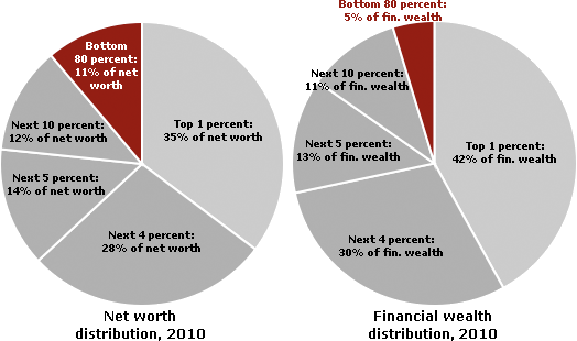
In the United States, wealth is highly concentrated in a relatively few hands. As of 2007, the top 1% of households (the upper class) owned 34.6% of all privately held wealth, and the next 19% (the managerial, professional, and small business stratum) had 50.5%, which means that just 20% of the people owned a remarkable 85%, leaving only 15% of the wealth for the bottom 80% (wage and salary workers). In terms of financial wealth (total net worth minus the value of one's home), the top 1% of households had an even greater share: 42.7%. Table 1 and Figure 1 present further details drawn from the careful work of economist Edward N. Wolff at New York University (2010).


Table 1: Distribution of net worth and financial wealth in theUnited States, 1983-2007
Total Net Worth
Top 1 percentNext 19 percentBottom 80 percent
198333.8%47.5%18.7%
198937.4%46.2%16.5%
199237.2%46.6%16.2%
199538.5%45.4%16.1%
199838.1%45.3%16.6%
200133.4%51.0%15.6%
200434.3%50.3%15.3%
200734.6%50.5%15.0%
Financial Wealth
Top 1 percentNext 19 percentBottom 80 percent
198342.9%48.4%8.7%
198946.9%46.5%6.6%
199245.6%46.7%7.7%
199547.2%45.9%7.0%
199847.3%43.6%9.1%
200139.7%51.5%8.7%
200442.2%50.3%7.5%
200742.7%50.3%7.0%

Total assets are defined as the sum of: (1) the gross value of owner-occupied housing; (2) other real estate owned by the household; (3) cash and demand deposits; (4) time and savings deposits, certificates of deposit, and money market accounts; (5) government bonds, corporate bonds, foreign bonds, and other financial securities; (6) the cash surrender value of life insurance plans; (7) the cash surrender value of pension plans, including IRAs, Keogh, and 401(k) plans; (8) corporate stock and mutual funds; (9) net equity in unincorporated businesses; and (10) equity in trust funds.

Total liabilities are the sum of: (1) mortgage debt; (2) consumer debt, including auto loans; and (3) other debt. From Wolff (2004, 2007, & 2010).


Figure 1: Net worth and financial wealth distribution in the U.S. in 2007

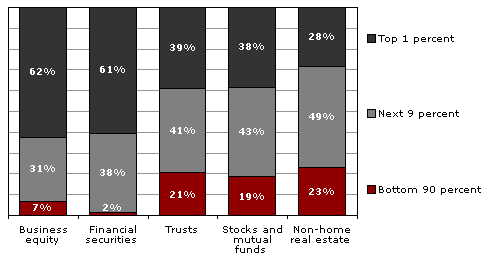
In terms of types of financial wealth, the top one percent of households have 38.3% of all privately held stock, 60.6% of financial securities, and 62.4% of business equity. The top 10% have 80% to 90% of stocks, bonds, trust funds, and business equity, and over 75% of non-home real estate. Since financial wealth is what counts as far as the control of income-producing assets, we can say that just 10% of the people own the United States of America.

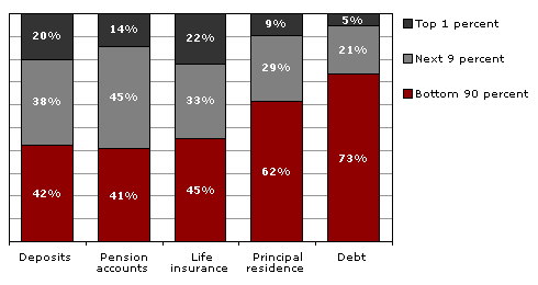
Table 2: Wealth distribution by type of asset, 2007
Investment Assets
Top 1 percentNext 9 percentBottom 90 percent
Business equity62.4%30.9%6.7%
Financial securities60.6%37.9%1.5%
Trusts38.9%40.5%20.6%
Stocks and mutual funds38.3%42.9%18.8%
Non-home real estate28.3%48.6%23.1%
TOTAL investment assets49.7%38.1%12.2%
Housing, Liquid Assets, Pension Assets, and Debt
Top 1 percentNext 9 percentBottom 90 percent
Deposits20.2%37.5%42.3%
Pension accounts14.4%44.8%40.8%
Life insurance22.0%32.9%45.1%
Principal residence9.4%29.2%61.5%
TOTAL other assets12.0%33.8%54.2%
Debt5.4%21.3%73.4%
From Wolff (2010).


Figure 2a: Wealth distribution by type of asset, 2007: investment assets

Figure 2b: Wealth distribution by type of asset, 2007: other assets
(...)


Table 3: Share of wealth held by the Bottom 99% and Top 1% in theUnited States, 1922-2007.
Bottom 99 percentTop 1 percent
192263.3%36.7%
192955.8%44.2%
193366.7%33.3%
193963.6%36.4%
194570.2%29.8%
194972.9%27.1%
195368.8%31.2%
196268.2%31.8%
196565.6%34.4%
196968.9%31.1%
197270.9%29.1%
197680.1%19.9%
197979.5%20.5%
198175.2%24.8%
198369.1%30.9%
198668.1%31.9%
198964.3%35.7%
199262.8%37.2%
199561.5%38.5%
199861.9%38.1%
200166.6%33.4%
200465.7%34.3%
200765.4%34.6%

Sources: 1922-1989 data from Wolff (1996). 1992-2007 data from Wolff (2010).
(...)

Here are some dramatic facts that sum up how the wealth distribution became even more concentrated between 1983 and 2004, in good part due to the tax cuts for the wealthy and the defeat of labor unions: Of all the new financial wealth created by the American economy in that 21-year-period, fully 42% of it went to the top 1%. A whopping 94% went to the top 20%, which of course means that the bottom 80% received only 6% of all the new financial wealth generated in the United States during the '80s, '90s, and early 2000s (Wolff, 2007).

(...)